Application 1:
Ligne haute tension → électrolyse des sels → ions.
V A B + V B C = V A − V B + V B − V C = V A − V C = V A C V_{A B}+V_{B C}=V_{A}-V_{B}+V_{B}-V_{C}=V_{A}-V_{C}=V_{A C} V A B + V BC = V A − V B + V B − V C = V A − V C = V A C Application 2:
1)
I 2 = I 0 − I 1 = 4 − 1 = 3 A I 5 = I 2 − I 4 = 3 − 2 = 1 A I 3 = I 1 + I 5 = 2 A \begin{aligned}
& I_{2}=I_{0}-I_{1}=4-1=3 \mathrm{~A} \\
& I_{5}=I_{2}-I_{4}=3-2=1 \mathrm{~A} \\
& I_{3}=I_{1}+I_{5}=2 \mathrm{~A}
\end{aligned} I 2 = I 0 − I 1 = 4 − 1 = 3 A I 5 = I 2 − I 4 = 3 − 2 = 1 A I 3 = I 1 + I 5 = 2 A Exercice à résoudre:
2) I = δ a q = e × e − I = e e − δ t I = = 1 ∂ t Pour + = + I e = 2 = 2 , I × 1 0 1 2 \text { 2) } \begin{aligned}
& I=\delta a \\
& q=e \times e^{-} \\
& I=e \frac{e^{-}}{\delta t} \\
& I==\frac{1}{\partial t} \\
& \text { Pour }+=+\frac{I}{e}=2=2, I \times 10^{\frac{1}{2}}
\end{aligned} 2) I = δ a q = e × e − I = e δ t e − I == ∂ t 1 Pour + = + e I = 2 = 2 , I × 1 0 2 1 Pendant dt:
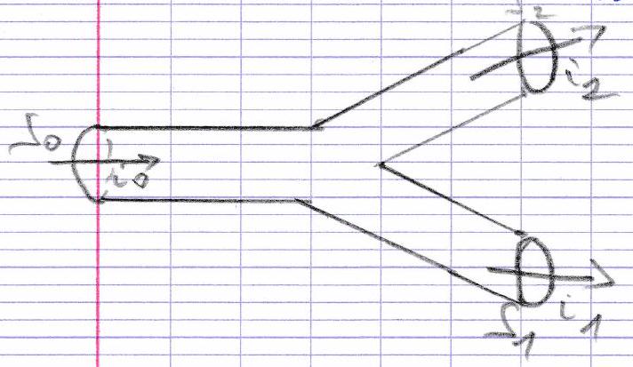
charge sortante par J 1 → d q 1 J_{1} \rightarrow d q_{1} J 1 → d q 1 S 2 → d q 2 S_{2} \rightarrow d q_{2} S 2 → d q 2 s 0 → d 0 s_{0} \rightarrow d_{0} s 0 → d 0 d q 0 = d q 1 + d q 2 ⇒ d q 0 d t = d q 1 d t + d q 2 d t ⇒ i 0 = i 1 + i 2 d q_{0}=d q_{1}+d q_{2} \Rightarrow \frac{d q_{0}}{d t}=\frac{d q_{1}}{d t}+\frac{d q_{2}}{d t} \Rightarrow i_{0}=i_{1}+i_{2} d q 0 = d q 1 + d q 2 ⇒ d t d q 0 = d t d q 1 + d t d q 2 ⇒ i 0 = i 1 + i 2
Applicationa:
E = U 1 U 2 = 0 U 2 = − U 1 + E = + 5 = − M 2 V E − U 1 + U 3 − U 4 = 0 U 3 = − E + U 1 + U 4 = − 5 + 3 + 1 = − 1 U U 1 = V A − V B U 3 = V B − V E E = V M − V A U 1 + U 3 = V A − V C E = 0 − V A V C = − 5 − U 1 − U 3 = − 5 = − 5 = − 5 = − 5 \begin{aligned}
& E=U_{1} U_{2}=0 \\
& U_{2}=-U_{1}+E=+5=-M_{2} V \\
& E-U_{1}+U_{3}-U_{4}=0 \\
& U_{3}=-E+U_{1}+U_{4}=-5+3+1=-1 U \\
& U_{1}=V_{A}-V_{B} \quad U_{3}=V_{B}-V E \quad E=V_{M}-V_{A} \\
& U_{1}+U_{3}=V_{A}-V_{C} \quad E=0-V_{A} \\
& V_{C}=-5-U_{1}-U_{3}=-5=-5=-5=-5
\end{aligned} E = U 1 U 2 = 0 U 2 = − U 1 + E = + 5 = − M 2 V E − U 1 + U 3 − U 4 = 0 U 3 = − E + U 1 + U 4 = − 5 + 3 + 1 = − 1 U U 1 = V A − V B U 3 = V B − V E E = V M − V A U 1 + U 3 = V A − V C E = 0 − V A V C = − 5 − U 1 − U 3 = − 5 = − 5 = − 5 = − 5 Application 4:
lompe: t cadiateur:- Eintale nuteris:Abouterio des provar tphowe:t
convention retepteur 1 retepteur, siciptater 3) P = Δ E Δ t Δ E = P × Δ F P=\frac{\Delta E}{\Delta t} \quad \Delta E=P \times \Delta F P = Δ t Δ E Δ E = P × Δ F
A N : Δ E = 1 × 1 0 3 × 1 × 3600 = 3 , 6 × 1 0 6 J A N: \Delta E=1 \times 10^{3} \times 1 \times 3600=3,6 \times 10^{6} \mathrm{~J} A N : Δ E = 1 × 1 0 3 × 1 × 3600 = 3 , 6 × 1 0 6 J Application 5
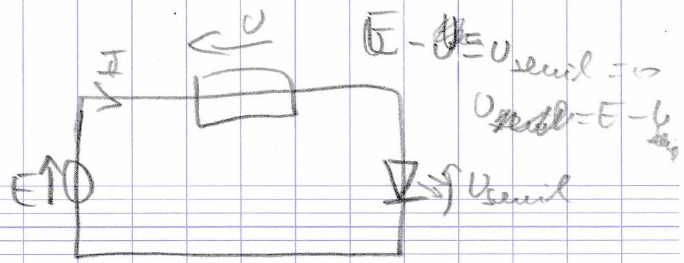
1 ∣ U = R I 1 \mid U=R I 1 ∣ U = R I I = I max I=I_{\text {max }} I = I max R = E − V sevil I max R=\frac{E-V_{\text {sevil }}}{I_{\text {max }}} R = I max E − V sevil R = 5 − 2 20 × 1 0 − 3 = 0 R=\frac{5-2}{20 \times 10^{-3}}=0 R = 20 × 1 0 − 3 5 − 2 = 0 15 × 1 0 2 Ω 15 \times 10^{2} \Omega 15 × 1 0 2 Ω 21 ρ = 2 r 0 × 20 × 1 0 − 3 = 4 , 0 × 1 0 − 2 W 21 \rho=2 r^{0} \times 20 \times 10^{-3}=4,0 \times 10^{-2} \mathrm{~W} 21 ρ = 2 r 0 × 20 × 1 0 − 3 = 4 , 0 × 1 0 − 2 W P − V = : x I max P-V=: x I_{\text {max }} P − V =: x I max
Or d’Opeí la loi d’ohm U = R X I max U = RX I_{\text{max}} U = RX I max Danc P = ℧ 2 R ˙ A N : P = 6 , 0 × 1 0 − 2 W \operatorname{Danc} P=\frac{\mho^{2}}{\dot{R}} \quad A N: P=6,0 \times 10^{-2} \mathrm{~W} Danc P = R ˙ ℧ 2 A N : P = 6 , 0 × 1 0 − 2 W P = U × I max P=U \times I_{\text {max }} P = U × I max V = R × I max V=R \times I_{\text {max }} V = R × I max P = R × I 2 P=R \times I^{2} P = R × I 2
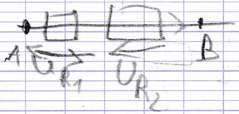
U R 1 = R 1 × I U R 2 = R 2 × I O 1 U R = U R 2 × U R 1 U R = I × ( R 1 + R 2 ) U R = R 21 × I R 21 = R 1 + R 2 \begin{gathered}
U_{R_{1}}=R_{1} \times I \\
U_{R_{2}}=R_{2} \times I \\
O_{1} U_{R}=U_{R_{2}} \times U_{R_{1}} \\
U_{R}=I \times\left(R_{1}+R_{2}\right) \\
U R=R_{21} \times I \\
R_{21}=R_{1}+R_{2}
\end{gathered} U R 1 = R 1 × I U R 2 = R 2 × I O 1 U R = U R 2 × U R 1 U R = I × ( R 1 + R 2 ) U R = R 21 × I R 21 = R 1 + R 2 U R 1 = R 1 × i 1 U R 2 = R 2 × i 2 i = U R 2 R 2 + U R 1 R 1 i = U R R iq U R R iq = U R 2 R 2 + U R 1 R 1 O r U R = U R 2 = U R 1 Dam Dam = 1 R iq = 1 R 2 + 1 R 1 \begin{gathered}
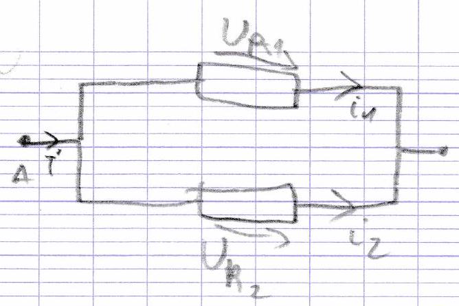
U_{R_{1}}=R_{1} \times i_{1} \\
U_{R_{2}}=R_{2} \times i_{2} \\
i=\frac{U_{R_{2}}}{R_{2}}+\frac{U R_{1}}{R_{1}} \\
i=\frac{U_{R}}{R_{\text {iq }}} \frac{U_{R}}{R_{\text {iq }}}=\frac{U_{R_{2}}}{R_{2}}+\frac{U R_{1}}{R_{1}} \\
O r U_{R}=U_{R_{2}}=U_{R_{1}} \\
\text { Dam } \\
\text { Dam }=\frac{1}{R_{\text {iq }}}=\frac{1}{R_{2}}+\frac{1}{R_{1}}
\end{gathered} U R 1 = R 1 × i 1 U R 2 = R 2 × i 2 i = R 2 U R 2 + R 1 U R 1 i = R iq U R R iq U R = R 2 U R 2 + R 1 U R 1 O r U R = U R 2 = U R 1 Dam Dam = R iq 1 = R 2 1 + R 1 1 Application 6