Chapitre ${ }^{9:}$ Appercation¶

Définition:¶

soit E, F deux ensembles. On appelle application de E vers F tout “mode de association” qui à tout élément de E associe un unique élément de F.

Notation $f: \left\lvert\, \begin{aligned} & \bar{E} \rightarrow F \\ & x \mapsto f(x)\end{aligned}\right.$

Vocabulaire:¶

• si $b=f(a)$, on dit que: 'b est l’image de a par f et a est un antécédent de b.

• Le graphe de $f$ est l’ensemble $\Gamma=\{(x, y) \in E \times F \mid y=f(x)\}$ ou encore $\Gamma=\{(x, f(x)) \mid x \in E\}$

• L’ensemble E est appelé ensemble de départ (ou source).

• L’ensemble F est appelé ensemble d’arrivée (ou but).

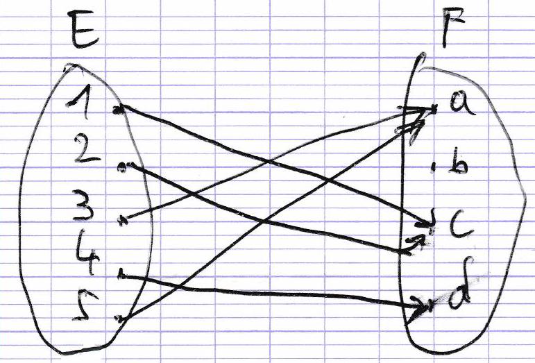
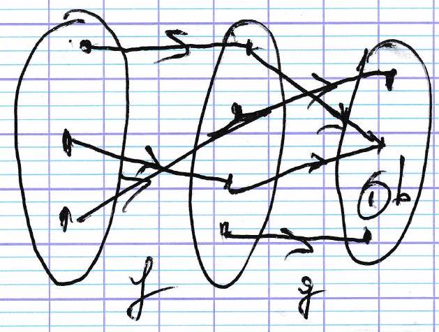
Représentation à l’aide d’un diagramme.

bon’ordre pas d’éléments parf c admet deux antécédents parf: Let 2 : d admet exactement un antécédent parf: 4

Égalité de deux applications. Soit $f: \left\lvert\, \begin{aligned} & E \rightarrow F \\ & x \mapsto f(x)\end{aligned}\right.$ et $g: \left\lvert\, \begin{aligned} & G \rightarrow H \\ & x \mapsto g(x)\end{aligned}\right.$ $f=g$ ssi $\left\{\begin{array}{l}E=b \\ F=H \\ \forall x \in E, f(x)=g(x)\end{array}\right.$

Application constante. $f: E \rightarrow F$ est dite constante si $(\forall x \in E)(\forall y \in E)(f(x)=f(y))$

Application indicatrice. Soit E un ensemble et A un sous-ensemble de E.

L’application indicatrice est définie par!

Propriété:¶

Soit $A, B$ deux sous-ensembles de $E$

a) $-\mathbb{1}_{\bar{A}}=1-\mathbb{1}_{A}$ b) $-\mathbb{1}_{A \cap B}=\mathbb{1}_{A} \mathbb{1}_{B}$ c) $-\mathbb{1}_{A \cup B}=\mathbb{1}_{A}+\mathbb{1}_{B}-\mathbb{1}_{A} \mathbb{1}_{B}$

Preuve: a) Soit $x \in E$

b) Soit $x \in E$

• dixtB:

donc: $\forall x \in E, \mathbb{1}_{A \cap B}(x)=\mathbb{1}_{A}(x) \mathbb{1}_{B}(x)$ c) $\overline{A \cup B}=\bar{A} \cap \bar{B} \quad \text{donc} \quad A \cup B=\bar{A} \cap \bar{B}$

Révision, prolongement: Soit $f: E \rightarrow F$ une application de $A$ un sous-ensemble de E. On appelle restriction de $f$ à A l’application notée $f \mid A$ $f_{\mid A}: \left\lvert\, \begin{aligned} & A \rightarrow F \\ & x \mapsto f(x)\end{aligned}\right.$ Soit $x$ un sous-ensemble de $E$ et $g: x \rightarrow F$ une application. On dit que $f$ est un prolongement de $g$ si $g=f_{\mid x}$

Exemple:¶

• exp: $\left\lvert\, \begin{aligned} & \mathbb{C} \rightarrow \mathbb{C} \\ & z \mapsto e^{z}\end{aligned}\right.$ est un prolongement de $\left\lvert\, \begin{aligned} & \mathbb{R} \rightarrow \mathbb{R} \\ & x \mapsto e^{x}\end{aligned}\right.$

• $\psi \left\lvert\, \begin{aligned} & \mathbb{C} \rightarrow \mathbb{R}^{+} \\ & z \mapsto|z|\end{aligned}\right.$ est un prolongement à $\mathbb{C}$ de $\left\lvert\, \begin{aligned} & \mathbb{R} \rightarrow \mathbb{R}^{+} \\ & z \mapsto|z|\end{aligned}\right.$

• $\left.S\right|_{z \mapsto \frac{e^{i z}+e^{-i z}}{2}} ^{\mathbb{C}}$ est un prolongement de $\cos$: $\left\lvert\, \begin{aligned} & \mathbb{R} \rightarrow \mathbb{R} \\ & x \mapsto \cos(x)\end{aligned}\right.$

Application induite: Soit $f: E \rightarrow E$ et $A$ un sous-ensemble de $E$. On dit que $A$ est stable par $f$ si

Dans ce cas, l’application induite par $f$ sur $A$ est l’application

Exemple: $f(x)=\sqrt{2+x}$ définie sur $]-2,+\infty[$ à valeurs dans $\mathbb{R}$. Pour tout $x \in I=[-2,+\infty[$

donc $f(x) \in I=[-2,+\infty[$

L’intervalle I est stable par $f$. La suite $\left(U_{n}\right)_{n \in \mathbb{N}}$ définie par $\left\{\begin{array}{l}u_{0} \in I \\ \forall n \in \mathbb{N}, u_{n+1}=f(u_{n})\end{array}\right.$

Image directe, image réciproque.

Soit $f: E \rightarrow F$, $X$ un sous-ensemble de $E$, $Y$ un sous-ensemble de $F$.

• L’image directe de $X$ par $f$ est l’ensemble $f(X)=\{f(x) \mid x \in X\}=\{y \in F \mid \exists x \in X, y=f(x)\}$

Exemples:

1. $f: \left\lvert\, \begin{aligned} & \mathbb{R} \rightarrow \mathbb{R} \\ & x \mapsto 0\end{aligned} \quad f([-1,3])=\{0\} \quad f(\mathbb{R})=\{0\}\right.$

2. $f: \left\lvert\, \begin{aligned} & \mathbb{R} \rightarrow \mathbb{R} \\ & x \mapsto x^{2}-4 x+3\end{aligned}\right.$

a) $f(\mathbb{R})=[-1,+\infty[$

a) Soit $x \in \mathbb{R}$

• Pour tout $x \in \mathbb{R}, f(x) \in[-1,+\infty[$: $f(\mathbb{R}) \subset [-1,+\infty[$

• Soit $y \in[-1,+\infty[$, alors $y+1 \geqslant 0$ $\Rightarrow y+1=(\sqrt{y+1})^{2}=(\sqrt{y+1}+2-2)^{2}$ Posons $x=\sqrt{y+1}+2$: $f(x)=-1+(x-2)^{2}=y$ Donc $y \in f(\mathbb{R})$ ainsi $[-1,+\infty[ \subset f(\mathbb{R})$ Donc $f(\mathbb{R})=[-1,+\infty[$

b) Soit $x \in[0,5]$ Alors $-2 \leq x-2 \leq 3$ puis $0 \leq(x-2)^{2} \leq 9$

donc $f(x) \in[-1,8]$: $f([0,5]) \subset[-1,8]$

Réciproquement, soit $y \in[-1,8]$

or $x=2+\sqrt{y+1}$ $0 \leq y \leqslant 9$ donc $0 \leq \sqrt{y+1} \leqslant 3$ donc $2 \leq x \leqslant 5$ donc $y \in f([0,5])$

c) $f$ est décroissante strictement sur $[-3,1]$ et continue donc d’après le théorème de la bijection réalise une bijection de $[-3,1]$ sur $[f(1), f(-3)] = [0,24]$

Ainsi: $f([-3,1])=[0,24]$

3. $f: \mathbb{C}^{*} \rightarrow \mathbb{C}$

Montrons que $f(U)=[-2,2]$

• Soit $z \in \mathbb{U}$

Or pour tout $z \in \mathbb{C}$, $\operatorname{Re}(z) \leqslant |z|$ donc $2 \operatorname{Re}(z) \leqslant 2$ donc $f(z) \in[-2,2]$ Ainsi $f(U) \subset[-2,2]$

Réciproquement, soit $y \in[-2,2]$¶

Il existe $\theta \in \mathbb{R}$ tel que $y=2 \cos(\theta)$ Alors $z=e^{i \theta} \in \mathbb{U}$

et $e^{i \theta} \in \mathbb{U}$. Ainsi: $[-2,2] \subset f(\mathbb{U})$

• L’image réciproque de $Y$ par $f$ est l’ensemble $f^{-1}(Y)=\{x \in E \mid f(x) \in Y\}$

Exemples:

1. $f: \left\lvert\, \begin{aligned} & \mathbb{R} \rightarrow \mathbb{R} \\ & x \mapsto x^{2}-4 x+3\end{aligned}\right.$

c) $x \in f^{-1}([-1 ; 8]) \Leftrightarrow 1 \leqslant f(x) \leq 8$

2. Soit $f: \mathbb{C}-\{-i\} \rightarrow \mathbb{C}$

a) $z \in f^{-1}(\mathbb{R}) \Leftrightarrow f(z) \in \mathbb{R}$

b) $z \in f^{-1}(\mathbb{R} i) \Leftrightarrow f(z) \in \mathbb{R} i$

$f^{-1}(\mathbb{R} i)=\mathbb{C}-\{-i\}$

Famille: Soit I un ensemble non vide et E un ensemble. On appelle famille de $E$ indexée par I toute application $\begin{aligned} I & \rightarrow E \\ i & \mapsto x\end{aligned}$

I: ensemble d’indices appelés indices. On la note $\left(x_{i}\right)_{i \in I}$

Dans le cas où $I=\mathbb{N}$, la famille est appelée suite d’éléments de $E$.

Exemples:¶

1. Pour tout $\alpha \in \mathbb{R}$, $f_{\alpha}: \mathbb{R} \rightarrow \mathbb{R}$, $x \mapsto e^{\alpha x}$

On dispose là d’une famille de fonctions indexée par $\mathbb{R}$.

2. Pour tout $r > 0$, $J_r = \left]-r, r\right[$. On dispose d’une famille d’intervalles : $\left(J_n\right)$.

Généralisation de $V, N$.

Soit $\left(A_i\right)_{i \in I}$ une famille de sous-ensembles d’un ensemble $E$.

Lois de De Morgan :

Partition d’un ensemble :

Soit $E$ un ensemble. Soit $\left\{ A_i \mid i \in I \right\}$ une famille de sous-ensembles de $E$.

Les sous-ensembles $A_i$ pour $i \in I$ forment une partition de $E$ si :

1. $\forall i \in I, A_i \neq \varnothing$

2. $(\forall i \in I)(\forall j \in I) \left( i \neq j \Rightarrow A_i \cap A_j = \varnothing \right)$

3. $E = \bigcup_{i \in I} A_i$

Exemples :¶

1. $\mathbb{Z}_2$ : ensemble des entiers pairs $2i$ ; ensemble des entiers impairs $\left\{ \mathbb{Z}_0, \mathbb{Z}_1 \right\}$ est une partition de $E$.

2. Soit $N \in \mathbb{N}^* - \{1\}$

$\mathbb{Z}_0, \mathbb{Z}_1, \ldots, \mathbb{Z}_{N-1}$ forment une partition de $\mathbb{Z}$.

• Soient $p, q$ deux entiers tels que : $0 \leqslant p \leqslant q \leqslant N-1$

Supposons $\mathbb{Z}_p \cap \mathbb{Z}_q \neq \varnothing$

Soit $x \in \mathbb{Z}_p \cap \mathbb{Z}_q$

$x \equiv p \pmod{N}$

et $x \equiv q \pmod{N}$

donc $p \equiv q \pmod{N}$

donc $q - p$ est un multiple entier de $N$

Or $0 \leqslant q - p \leqslant N - 1$ donc $q - p = 0$

Par contraposée, si $p \neq q$ alors $\mathbb{Z}_p \cap \mathbb{Z}_q = \varnothing$

• $\forall k \in \llbracket 0, N-1 \rrbracket, \mathbb{Z}_k \subset \mathbb{Z}$ donc $\bigcup_{k=0}^{N-1} \mathbb{Z}_k \subset \mathbb{Z}$

Réciproquement, soit $x \in \mathbb{Z}$

Par division euclidienne de $x$ par $N$, il existe $q \in \mathbb{Z}$ et $r \in \llbracket 0, N-1 \rrbracket$ tels que : $x = Nq + r$

donc $x \in \mathbb{Z}_r$

Ce qui montre que $\mathbb{Z} \subset \bigcup_{k=0}^{N-1} \mathbb{Z}_k$

Par double inclusion :

$\mathbb{Z} = \bigcup_{k=0}^{N-1} \mathbb{Z}_k$

$\mathbb{Z}_k$ : classe des entiers congrus à $k$ modulo $N$

3. $\mathbb{Q}, \mathbb{R} - \mathbb{Q}$ forment une partition de $\mathbb{R}$

Application injective, surjective, bijective

Soit $f: E \rightarrow F$

On s’intéresse à l’équation $f(x) = b$ où $b \in F$.

On note $N(b)$ le nombre de solutions de l’équation $f(x) = b$.

• Si : $\forall b \in F, N(b) = 1$

On dit que $f$ est une bijection.

• Si : $\forall b \in F, N(b) = 0$ ou $N(b) = 1$

C’est-à-dire tout élément $b \in F$ admet au plus un antécédent dans $E$, on dira que $f$ est injective.

• Si : $\forall b \in F, N(b) \geqslant 1$ c’est-à-dire tout élément $b \in F$ admet au moins un antécédent dans $E$, on dira que $f$ est surjective.

Définition : Soit $f: E \rightarrow F$

• On dit que $f$ est surjective de $E$ dans $F$ si : $\forall y \in F, \exists x \in E, y = f(x)$

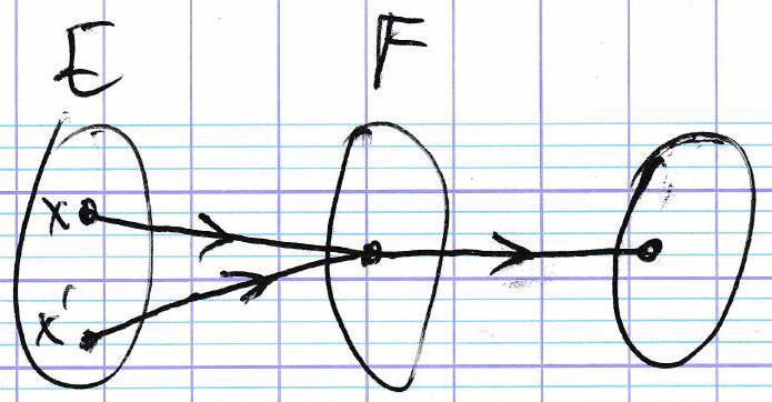
• On dit que $f$ est injective de $E$ dans $F$ si : $(\forall x \in E)(\forall x' \in E)(x \neq x' \Rightarrow f(x) \neq f(x'))$

cad : $(\forall x \in E)(\forall x' \in E)(f(x) = f(x') \Rightarrow x = x')$

• On dit que $f$ est bijective de $E$ dans $F$ si :

$(\forall y \in F)(\exists! x \in E)(y = f(x))$

càd si $f$ est à la fois injective et surjective.

Exemples :¶

1. $\operatorname{id}_E \left\lvert\, \begin{aligned} & E \rightarrow E \\ & x \mapsto x \end{aligned} \right.$ est une bijection.

2. $f_1: \left\lvert\, \begin{aligned} & \mathbb{R} \rightarrow \mathbb{R} \\ & x \mapsto x^2 \end{aligned} \right.$ ni injective, ni surjective.

$f_2: \left\lvert\, \begin{aligned} & \mathbb{R} \rightarrow \mathbb{R}^+ \\ & x \mapsto x^2 \end{aligned} \right.$ surjective, non injective.

$f_3: \left\lvert\, \begin{aligned} & \mathbb{R}^+ \rightarrow \mathbb{R}^+ \\ & x \mapsto x^2 \end{aligned} \right.$ bijective.

3. $f_1: \left\lvert\, \begin{aligned} & \mathbb{R} \rightarrow \mathbb{R} \\ & x \mapsto \cos(x) \end{aligned} \right.$ ni injective, ni surjective.

$f_2: \left\lvert\, \begin{aligned} & \mathbb{R} \rightarrow \left[-1, 1\right] \\ & x \mapsto \cos(x) \end{aligned} \right.$ non injective, surjective.

$f_3: \left\lvert\, \begin{aligned} & \mathbb{R} \rightarrow \mathbb{R} \\ & x \mapsto \cos(x) \end{aligned} \right.$ ni injective, ni surjective.

3. $f: \left\lvert\, \begin{aligned} & \mathbb{C} \rightarrow \mathbb{C} \\ & z \mapsto z^2 + z \end{aligned} \right.$

Injective : En effet, pour tout $b \in \mathbb{C}$, l’équation $z^2 + z = b$ admet toujours une solution.

Non injective : $f(0) = f(-1)$

4. $f: \left\lvert\, \begin{aligned} & P(E) \rightarrow P(E) \\ & X \mapsto \overline{X} \end{aligned} \right.$ bijective.

Soit $B \in P(E)$

$\varphi$ est bijective et $\varphi^{-1} = \varphi$ (involution).

Définition :

Soit $f: E \rightarrow F$ une bijection.

L’application $\begin{array}{l} F \rightarrow E \\ y \mapsto \text{ l'antécédent de } y \text{ par } f \end{array}$ est appelée application réciproque de $f$, et on la note $f^{-1}$.

On a l’équivalence :

Propriétés vis-à-vis de la composition :

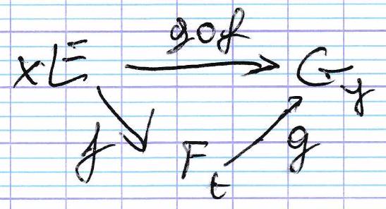
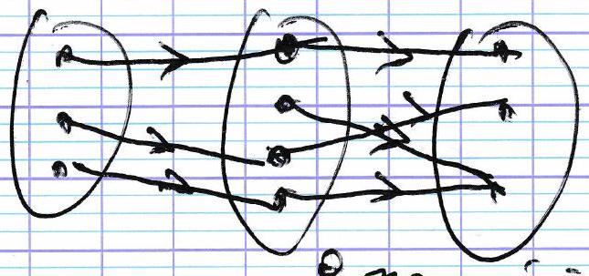
Soit $f: E \rightarrow F$ et $g: F \rightarrow G$

1. Si $f$ et $g$ sont injectives, alors $g \circ f$ est injective.

2. Si $f$ et $g$ sont surjectives, alors $g \circ f$ est surjective.

3. Si $f$ et $g$ sont bijectives, alors $g \circ f$ est bijective.

Preuve :

1. Supposons $f$ et $g$ injectives. Montrons que $g \circ f$ est injective.

Soit $x, x' \in E$ tels que $g \circ f(x) = g \circ f(x')$

Alors $g(f(x)) = g(f(x'))$

Or $g$ est injective donc $f(x) = f(x')$

De nouveau, $f$ est injective donc $x = x'$

2. Supposons $f$ et $g$ surjectives.

Soit $y \in G$

Par surjectivité de $g$, il existe $t \in F$ tel que $y = g(t)$

Par surjectivité de $f$, il existe $x \in E$ tel que $t = f(x)$

Alors $y = g(f(x)) = g \circ f(x)$

3. Résulte de 1) et 2)

Propriétés :

Soit $f: E \rightarrow F$, $g: F \rightarrow G$ bijectives.

Alors $(g \circ f)^{-1} = f^{-1} \circ g^{-1}$

Preuve :

Soit $y \in G$, $x \in E$

Que peut-on dire si $g \circ f$ est injective ? Que peut-on dire si $g \circ f$ est surjective ?

Si $f$ n’est pas injective, alors $g \circ f$ n’est pas injective. Donc par contraposée, si $g \circ f$ est injective, alors $f$ est injective.

$g$ non injective

alors $g \circ f$ non injective

Si $g \circ f$ est injective, alors $f$ est injective, mais on ne peut rien dire de $g$.

Exemple : $f: \mathbb{R}^+ \rightarrow \mathbb{R}^+$, $x \mapsto \sqrt{x}$, $g: \mathbb{R} \rightarrow \mathbb{R}^+$, $x \mapsto x^2$

$g \circ f: \mathbb{R}^+ \rightarrow \mathbb{R}^+$, $x \mapsto x$ est injective, mais $g$ n’est pas injective car $g(-1) = g(1)$.

Si $f$ n’est pas surjective, alors $g \circ f$ n’est pas surjective. Donc par contraposée, si $g \circ f$ est surjective, alors $f$ est surjective.

Si $f$ n’est pas surjective, alors $g \circ f$ n’est pas surjective. Donc par contraposée, si $g \circ f$ est surjective, alors $f$ est surjective.

Exemple : $f: \mathbb{R}^+ \rightarrow \mathbb{R}^2$, $g: \mathbb{R} \rightarrow \mathbb{R}^+$, $x \mapsto x^2$

$g \circ f: \mathbb{R}^+ \rightarrow \mathbb{R}^+$, $x \mapsto x^2$ est surjective, mais $f$ n’est pas surjective.

Propriétés :

Soit $f: E \rightarrow F$, $g: F \rightarrow G$

1. Si $g \circ f$ est injective, alors $f$ est injective.

2. Si $g \circ f$ est surjective, alors $g$ est surjective.

Preuve :

1. Supposons $g \circ f$ injective.

Montrons que $f$ est injective.

Soit $x, x' \in E$ tels que $f(x) = f(x')$

Alors $g \circ f(x) = g \circ f(x')$

Or $g \circ f$ est injective donc $x = x'$

Ainsi $f$ est injective.

2. Supposons $g \circ f$ surjective.

Montrons que $g$ est surjective.

Soit $y \in G$

Il existe $x \in E$ tel que $g \circ f(x) = y$

Alors $y = g(f(x))$ donc $f(x)$ est un antécédent de $y$ par $g$.

Ainsi $g$ est surjective.

Réciproque : soit $f: E \rightarrow F$

$f$ est bijective si :

$\exists h: F \rightarrow E$ telle que $f \circ h = \text{id}_F$ et $h \circ f = \text{id}_E$

Dans ce cas, $h = f^{-1}$

Preuve :¶

• Montrons que la condition est nécessaire. Supposons $f$ bijective. Il suffit de prouver $h = f^{-1}$.

• Montrons que la condition est suffisante. Supposons qu’il existe $h: F \rightarrow E$ telle que $f \circ h = \text{id}_F$ et $h \circ f = \text{id}_E$.

• $\text{id}_F$ est surjective donc $f \circ h$ est surjective donc $f$ est surjective.

• $\text{id}_E$ est injective donc $h \circ f$ est injective donc $f$ est injective.

Donc $f$ est bijective.

I est injective, Aind is fastbijective